Computing properties of a quarter circle
This is an example of how to compute some properties of a circular section like area, inertia and its centroid, using finite element method.
First step
The first step when programming with Python is always import the libraries we will use. In this example two libraries are required
# Libraries
import numpy as np
import matplotlib.pyplot as plt
Second step
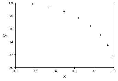
Next we define the number of nodes to approximate the circular section and the coordinate matrix, where we store the number of each node and its position in the Cartesian coordinates. In this matrix the first node will be always at the origin, while the others will be equally distributed on the perimeter of the quarter circle. This code can be written as
nnos = 11                  # number of nodes
nel  = nnos - 2            # number of elements
coord = np.zeros((nnos,3))  # coordinate matrix pre-allocation
coord[0][0] = 1
theta = (np.pi/2)/(nnos - 2) # theta value
for i in range(0, nnos - 1):
   coord[i + 1][0] = i + 2          # Number of node
   coord[i + 1][1] = np.cos(theta*i) # X coordinate
   coord[i + 1][2] = np.sin(theta*i) # Y coordinate

# Scatter
fig = plt.figure()
plt.xlim([0, 1])
plt.ylim([0, 1])
plt.scatter(coord[:,1], coord[:,2], marker = '+', c = 'black')
plt.xlabel('x', fontsize = 'xx-large')
plt.ylabel('y', fontsize = 'xx-large')
Third step
The following step is defining the elements. This definition is carried in the incidence matrix, where we establish the set of nodes which constitute each element. We can notice in the Figure below that all elements share the node at the origin, therefore we can write the incidence matrix as
# incidence matrix pre-allocation
inci = np.zeros((nel, 3))

for i in range(0, nel):
   #central node
   inci[i][0] = 1
   # second node
   inci[i][1] = i + 2
   # third node
   inci[i][2] = i + 3
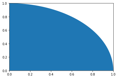
The simplest way to plot these set of elements is
fig, ax = plt.subplots()
plt.xlim([0,1])
plt.ylim([0,1])
ax.fill(coord[:, 1], coord[:,2], 'b')
This Python code above plots all elements in blue as illustrated in the first Figure. If you want to plot each element separately as illustrated in the Figure below, you should write the following code
fig, ax = plt.subplots()
 plt.xlim([0,1])
 plt.ylim([0,1])
 for i in range(0, nel):
    # set of nodes
    node1 = inci[i][0]
    node2 = inci[i][1]
    node3 = inci[i][2]

    # x-axis position
    x1 = coord[int(node1) - 1][1]
    x2 = coord[int(node2) - 1][1]
    x3 = coord[int(node3) - 1][1]
    x  = np.array([x1, x2, x3])

    # y-axis position
    y1 = coord[int(node1) - 1][2]
    y2 = coord[int(node2) - 1][2]
    y3 = coord[int(node3) - 1][2]
    y  = np.array([y1, y2, y3])

    if i%2 == 0:
       ax.fill(x, y,'k',alpha=0.3)
    else:
       ax.fill(x, y,'b',alpha=0.3)
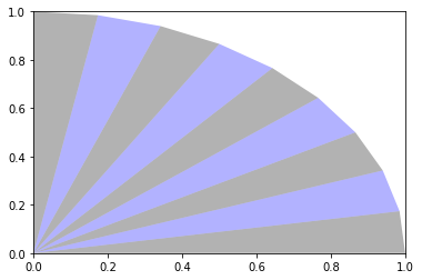
Fourth step
Next we compute the area of the section illustrated in the Figure above. The strategy in this example is divide the circular section area in many triangular elements. We compute the area of a single element and sum all of them to have the total area. From analytic geometry, we know how to compute the area of any triangle. Taking these information in consideration we can write the Python code as
A = 0 # summation variable pre-allocation

# central node coordinates
x1 = coord[int(inci[0,0] - 1), 1]
y1 = coord[int(inci[0,0] - 1), 2]

for i in range(0, nel):
    # second node coordinates
    x2 = coord[int(inci[i,1] - 1), 1]
    y2 = coord[int(inci[i,1] - 1), 2]

    # third node coordinates
    x3 = coord[int(inci[i,2] - 1), 1]
    y3 = coord[int(inci[i,2] - 1), 2]

    # area of a single element
    a = 0.5*((x2 - x1)*(y3-y1) - (x3 - x1)*(y2 - y1))

    # area summation
    A +=a

# relative error
error_area = (np.pi/4 - A)/(np.pi/4)*100

# print error
print('Error = ', error_area,'%')
Using only 9 elements the error of the area is around 0,51%.
Next we want to evaluate the centroid of our section area with the following Python code
centx = 0 # centroid in X-axis pre-allocation
centy = 0 # centroid in Y-axis pre-allocation

# central node coordinates
x1 = coord[int(inci[0,0] - 1), 1]
y1 = coord[int(inci[0,0] - 1), 2]

for i in range(0,nel):
    #     second node coordinates
    x2 = coord[int(inci[i,1] - 1), 1]
    y2 = coord[int(inci[i,1] - 1), 2]

    #     third node coordinates
    x3 = coord[int(inci[i,2] - 1), 1]
    y3 = coord[int(inci[i,2] - 1), 2]

    # area of a single element
    a = 0.5*((x2 - x1)*(y3-y1) - (x3 - x1)*(y2 - y1))

    # centroid summation
    centx += a*((x1+x2+x3)/3)
    centy += a*((y1+y2+y3)/3)

X = centx/A              # centroid in X-axis
Y = centy/A              # centroid in Y-axis

exact_cent = 4/(np.pi*3) # exact centroid

error_x = (exact_cent - X)/exact_cent*100 # relative error X-axis
error_y = (exact_cent - Y)/exact_cent*100 # relative error Y-axis

# print relative error in both axis
print('Error centroid X = ', error_x,'%')
print('Error centroid Y = ', error_y,'%')
Using only 9 elements the centroid relative error is around 0,25%.
The last property we want to compute is the moment of inertia of a quarter circle. For this we will use the Python code below
Ix = 0 # moment of inertia in X-axis pre-allocation
Iy = 0 # moment of inertia in Y-axis pre-allocation

# central node coordinates
x1 = coord[int(inci[0,0] - 1), 1]
y1 = coord[int(inci[0,0] - 1), 2]

for i in range(0,nel):
    #     second node coordinates
    x2 = coord[int(inci[i,1] - 1), 1]
    y2 = coord[int(inci[i,1] - 1), 2]

    #     third node coordinates
    x3 = coord[int(inci[i,2] - 1), 1]
    y3 = coord[int(inci[i,2] - 1), 2]

    # moment of inertia summation
    Ix += 1/12*(y1**2+y2**2+y3**2+y1*y2+y1*y3+y2*y3)*(x2*y3-x3*y2)
    Iy += 1/12*(x1**2+x1*x2+x1*x3+x2**2+x2*x3+x3**2)*(x2*y3-x3*y2)

# exact value of the moment of inertia
Iexact = np.pi/16

# relative error
error_Ix = (Iexact-Ix)/Iexact*100
error_Iy = (Iexact-Iy)/Iexact*100

# print relative error
print('Error inertia X = ', error_Ix,'%')
print('Error inertia Y = ', error_Iy,'%')
Using only 9 elements the moment of inertia relative error is around 1,01%.
If you desire a better approximation increase the number of nodes at the second step.